
ECR Now Allows 200 GB Image Layers. Your Model Weights Still Do Not Belong There

On August 3, 2026, AWS raised the maximum Amazon ECR image layer size to 200 GB for images pushed with docker push. The announcement names the driver in the second paragraph: “embedding large language models, bundling genomics datasets, or packaging large binary dependencies directly into your container images.” Nobody asked for a 200 GB layer to ship a Go binary. Teams asked for it because they were trying to COPY a checkpoint directory into an image and hitting a wall.
The wall was real. The fix is real. And for most inference workloads, using it is still the wrong call.
That is not a contrarian pose. It matches what AWS itself publishes in the EKS Best Practices Guide, which ranks the options for handling model artifacts “from least to most recommended” and puts “baking the model into the container image” at the bottom of the list. AWS raised a quota because customers kept hitting it. That is a support-ticket decision, not an architecture endorsement.
This article covers the old limit and why it broke model-in-image builds, what a fat layer actually costs in storage, transfer, and pod startup, why a single 200 GB layer defeats every deduplication and caching mechanism in the container ecosystem, how SOCI and node-side caching change the math, and a decision framework for choosing between weights-in-image, S3 plus a mount, and a shared filesystem. There is also a short list of cases where a 200 GB layer genuinely is the right answer.
What the limit was, and what it is now
The old ceiling was 52,000 MiB. That is the value still published on the ECR service quotas page as of this writing, listed as “Maximum layer size, Each supported Region: 52,000” and marked not adjustable. 52,000 MiB works out to roughly 50.8 GiB, or about 54.5 GB in decimal units. Close enough to “50 gigabytes” that everyone rounded it that way in their heads.
The new limit splits by push path, and this is the part people are going to trip over.
| Push path | Maximum layer size | Source |
|---|---|---|
docker push (Docker Registry HTTP API v2) |
200 GB | AWS What’s New, Aug 3 2026 |
AWS SDK or CLI via UploadLayerPart |
50 GB | AWS What’s New, Aug 3 2026 |
Documented quota value (Maximum layer size) |
52,000 MiB | ECR service quotas |
Layer parts count, API multipart path |
4,200 | ECR service quotas |
Maximum layer part size, API multipart path |
10 MiB | ECR service quotas |
Multiply the last two rows and you get 42,000 MiB, roughly 41 GiB. The documented multipart ceiling is therefore lower than the documented layer size quota, and lower again than the 50 GB the announcement attributes to the SDK path. I could not reconcile those three numbers from public documentation, and the quotas page has not been updated for the launch. Treat the 200 GB figure as applying only to the docker push code path until the quotas page catches up, and test your own pipeline rather than trusting arithmetic. If your CI uses the ECR API directly instead of a Docker-compatible client, you are on the lower limit and you may be on the lowest of the three.
One more constraint from the announcement: the increase is live in every AWS Region and partition where ECR runs, except Middle East (Bahrain) and Middle East (UAE). If you build once and replicate broadly, that pair will reject the push.
Why model-in-image builds hit the ceiling in the first place
A Dockerfile instruction produces one layer. COPY ./model /opt/model produces exactly one layer containing the entire directory tree, serialized as a tar archive and typically gzip-compressed. That is not a Docker implementation detail you can argue with. It is how the OCI image layer specification defines a filesystem changeset: one blob, one media type such as application/vnd.oci.image.layer.v1.tar+gzip, addressed by the digest of its content.
So a checkpoint directory of 180 GB becomes a single 180 GB blob. There is no automatic sharding. Under the old 52,000 MiB limit, the push failed, and the workaround was to split the copy across multiple instructions by hand:
# The pre-August-2026 workaround: manual sharding to stay under ~50 GB per layer
COPY model/shard-00/ /opt/model/shard-00/
COPY model/shard-01/ /opt/model/shard-01/
COPY model/shard-02/ /opt/model/shard-02/
COPY model/shard-03/ /opt/model/shard-03/
That is ugly, it is brittle when shard counts change between model revisions, and it means your Dockerfile encodes the physical layout of a checkpoint. Teams hated it. Fair enough.
Model weights make the problem worse than a generic large payload because they barely compress. Safetensors and similar formats store dense float16 or bfloat16 tensors. gzip on that data returns a few percent at best, so compressed layer size tracks on-disk size almost one to one. Every optimization instinct you developed compressing Python wheels and Debian packages stops helping here.
The frameworks are not small either. AWS documents pytorch/pytorch:2.7.1-cuda11.8-cudnn9-runtime at 3.03 GB against 6.66 GB for the devel variant, per the EKS Best Practices Guide. That is before a single weight file. Add CUDA libraries, an inference server, and a 140 GB checkpoint and you are looking at an image where 97% of the bytes are one immutable artifact that has nothing to do with your code.
What a fat layer actually costs
Storage is the cheap part, and people fixate on it anyway. ECR private repository storage runs $0.10 per GB-month, per the ECR pricing page. A 200 GB image is $20 a month. Nobody is going to escalate that.
The bill gets interesting when you count revisions. Because layers are content-addressed, changing one byte inside a layer produces a new digest and a completely new blob. ECR stores both. If your pipeline rebuilds an image with weights baked in and you keep thirty tagged revisions for rollback, you are paying for thirty copies of the same weights unless the weights layer digest is byte-identical across all of them.
| Scenario | Stored bytes | ECR storage cost per month |
|---|---|---|
| One 200 GB image, single revision | 200 GB | $20.00 |
| 200 GB image, 10 revisions, weights layer unchanged | 200 GB + 10 x 5 GB code layers = 250 GB | $25.00 |
| 200 GB image, 10 revisions, weights layer rebuilt each time | 2,000 GB | $200.00 |
| Thin 5 GB image, 10 revisions, weights in S3 Standard | 50 GB ECR + 195 GB S3 | $5.00 + $4.49 = $9.49 |
Storage rates: ECR private repositories at $0.10 per GB-month and S3 Standard at $0.023 per GB-month for the first 50 TB, both from the ECR pricing page and S3 pricing page, us-east-1, August 2026. The 10-revision rows assume no lifecycle expiry.
Row three is the one that bites. A rebuilt weights layer is the default outcome, not an edge case, because COPY layer digests depend on file mtimes and ordering unless you are deliberate about reproducibility. One careless git clone of the model repo in CI and every build produces a fresh 195 GB blob.
Data transfer is free in the direction that matters most. Pulls from ECR to EC2, ECS, Fargate, or Lambda in the same Region cost nothing, which the pricing page states explicitly and reinforces with a worked example where 1 TB of in-Region pulls is billed at $0.00. Cross-Region is where it stops being free. The same page’s second pricing example charges $0.09 per GB for pulls into a different Region. Replicate a 200 GB image into three additional Regions and you pay $18 per Region per replication event, plus storage in each destination.
The real cost is time. That is what shows up in your latency graphs, your GPU utilization, and your on-call rotation.
Pull time is where the 200 GB layer actually hurts
Container image pull is the dominant term in AI inference cold start. AWS states this directly in the ai-on-eks cold start guidance: “Container image pull time is a primary contributor to the startup latency of AI/ML inference applications.”
Pull has two phases, and a single giant layer sabotages both.
Phase one is fetching bytes from the registry. containerd downloads multiple layers concurrently, but a single layer is a single HTTP GET against one blob. One TCP stream, one connection, one throughput ceiling. AWS describes exactly why SOCI’s parallel mode exists: it “creates multiple concurrent HTTP connections per layer, multiplying download throughput beyond the single-connection limitation.” That limitation is the default behavior you get without SOCI.
Phase two is decompression and unpacking. A gzip stream is inherently sequential. You cannot decompress the middle of a gzip member without processing everything before it. One 200 GB layer is one gzip stream, which means one decompression thread, which means one CPU core doing all the work while the other 191 cores on your p5.48xlarge sit idle. SOCI’s parallel unpack “processes multiple layers simultaneously,” using available cores to decompress and extract concurrently. Multiple layers. A single layer has nothing to parallelize across.
Here is modeled arithmetic for a 200 GB payload. These are calculations from assumed throughput figures, not benchmark results, and your numbers will differ with instance type, Region, and time of day. The point is the shape of the curve, not the absolute values.
| Layout | Fetch concurrency | Assumed effective throughput | Modeled fetch time | Unpack parallelism |
|---|---|---|---|---|
| One 200 GB layer, containerd default | 1 connection | 400 MB/s | 8 min 20 s | 1 core |
| One 200 GB layer, SOCI parallel pull | 8 connections | 2.4 GB/s | 1 min 23 s | still 1 core |
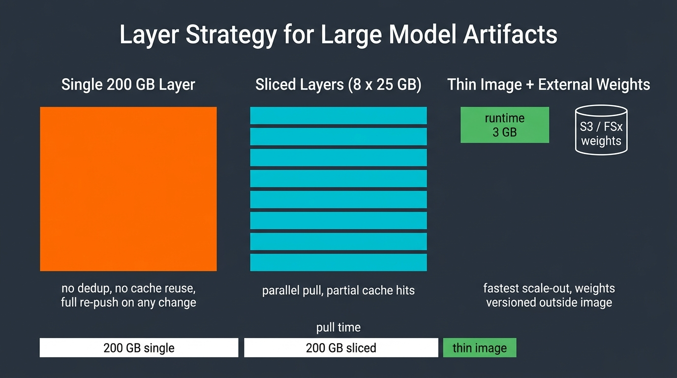
| 8 x 25 GB layers, containerd default | 3 concurrent layers | 1.2 GB/s | 2 min 46 s | up to 3 cores |
| 8 x 25 GB layers, SOCI parallel pull and unpack | 8 layers x 4 connections | 6 GB/s | 33 s | up to 8 cores |
| 3 GB runtime image, weights from S3 at 3 GB/s | 3 concurrent layers | 1.2 GB/s image | 2.5 s image + 66 s weights | not applicable to weights |
Assumptions: containerd’s default max_concurrent_downloads is 3; per-connection registry throughput of 400 MB/s; aggregate ENA bandwidth sufficient to absorb the parallel cases; model weights treated as incompressible so compressed size equals on-disk size. Decompression time is excluded from the fetch column and discussed separately.
Two things fall out of that table. First, SOCI parallel pull rescues the single-layer case for fetch but does nothing for unpack, so the giant layer still serializes on one core during extraction. Second, the thin image plus external weights row wins on total time even before you account for the fact that S3 reads can be resumed, ranged, and parallelized far more aggressively than a registry blob.
Scale-out multiplies all of this. Twenty pods landing on twenty fresh nodes during a traffic spike means twenty independent 200 GB pulls. In-Region transfer is free, so there is no bill, but there is a Region-level GetDownloadUrlForLayer quota of 3,000 requests per second and a BatchGetImage quota of 2,000 per second per the quotas page. Those are per-layer and per-image calls, not per-byte, so a fat-layer image is actually API-frugal. What it is not is fast. Your autoscaler decision at T+0 becomes a serving pod at T+9 minutes, and Karpenter cannot help you because the node was ready in 45 seconds and then sat there downloading.
The first community reaction I saw to the announcement went straight to this point. A Japanese developer posted on August 5 asking whether a 200 GB image would blow past Lambda’s 15-minute ceiling on the pull alone. Wrong service, since Lambda images are still capped at 10 GB, but exactly the right instinct: the interesting number in this launch is not gigabytes, it is seconds.
Why one giant layer defeats deduplication and caching
Container registries deduplicate at layer granularity. That is the whole design. The OCI image spec defines each layer as a blob identified by the digest of its content, and every consumer in the chain uses that digest as a cache key: ECR checks BatchCheckLayerAvailability before uploading, containerd checks its local content store before downloading, and BuildKit checks its cache before rebuilding.
Layer granularity means the granularity of reuse is the granularity of your layers. Make one layer that is 97% of your image and you have opted out of the mechanism.
Concretely, here is what breaks.
Push deduplication stops working. ECR skips uploading a layer whose digest already exists. With weights and code in the same layer, any code change produces a new digest for the whole 200 GB blob, and you re-upload all of it. The quotas page notes that BatchCheckLayerAvailability runs per layer during push specifically so previously uploaded layers get skipped. You get one check, it misses, and you push 200 GB.
Node cache reuse stops working. A node that already has the previous revision of your image holds the old 200 GB blob. The new revision shares nothing with it. The node downloads 200 GB again and now holds 400 GB of near-identical bytes until garbage collection runs. If instead your weights sit in their own layer and your code sits in another, the node reuses the weights blob and pulls a few megabytes.
Build cache reuse stops working. BuildKit caches per instruction. One COPY that ingests 195 GB is one cache entry that invalidates wholesale.
Lifecycle policy math gets awkward. ECR lifecycle policies expire images, not layers, and a layer survives as long as any image references it. Untagged image expiry is the standard cost control, and it works, but with a monolithic layer you cannot expire the stale weights while keeping recent code revisions. They are the same object.
Cross-Region replication gets expensive per event. Because replication copies layers, an unchanged weights layer replicates once and is skipped thereafter. A rebuilt monolithic layer replicates in full every time, at $0.09 per GB per the pricing page. The ECR pull-through cache and referrer discovery behavior has the same property: caches are populated per layer, so a monolithic layer is a cache entry that either hits completely or misses completely, with no partial warmth.
None of this is new. It is the same argument for ordering Dockerfile instructions from least to most volatile, which is the core discipline behind multi-stage Docker builds. The 200 GB limit just raised the stakes on getting it wrong.
Layer strategy when you insist on shipping the weights
Suppose you have decided the weights go in the image. There are legitimate reasons, covered later. Do it carefully.
Split by change frequency, not by convenience. Base OS, CUDA runtime, Python dependencies, inference server, and model weights all change on different schedules. Give each its own layer, ordered from most stable to most volatile:
# syntax=docker/dockerfile:1.7
FROM nvcr.io/nvidia/pytorch:26.06-py3 AS runtime

# Layer: Python deps. Changes weekly.
COPY requirements.lock /tmp/
RUN --mount=type=cache,target=/root/.cache/pip \
    pip install --require-hashes -r /tmp/requirements.lock

# Layer: inference server code. Changes daily.
COPY --link server/ /opt/server/

# Layers: weights, sliced. Changes per model release only.
# One COPY per shard group keeps each layer well under the limit
# and lets containerd fetch them concurrently.
COPY --link weights/group-a/ /opt/model/
COPY --link weights/group-b/ /opt/model/
COPY --link weights/group-c/ /opt/model/
COPY --link weights/group-d/ /opt/model/
COPY --link matters here. It creates the layer independently of the parent chain, so a change in an earlier layer does not invalidate later ones. Without it, editing requirements.lock invalidates every subsequent COPY, including all four weight layers.
Target 20 to 30 GB per weights layer. That gives containerd’s default three concurrent downloads something to work with, keeps each gzip stream small enough that decompression on one core is not the wall clock, and stays comfortably inside every documented quota including the API multipart path. Eight layers of 25 GB is a better 200 GB image than one layer of 200 GB in every dimension except Dockerfile line count.
Make the weights layer reproducible. If the digest changes on every build, you have gained nothing:
# Normalize mtimes so identical content produces an identical layer digest
find weights/ -exec touch -t 200001010000 {} +

# Verify the digest is stable across builds
docker buildx build --output=type=image,push=false -t model:probe .
docker image inspect model:probe --format '' | jq -r '.[]'
Run that twice from a clean checkout. If the weights layer digests differ, find the source of nondeterminism before you ship, or you will pay row three of the storage table every single build.
Consider zstd. The OCI spec defines application/vnd.oci.image.layer.v1.tar+zstd alongside the gzip media type, and zstd decompresses substantially faster than gzip. On incompressible weight data the compression ratio is a wash, so you are buying decompression speed, not smaller blobs. Verify your runtime accepts zstd layers before switching. containerd does; some older tooling in your supply chain may not.
Finally, push from a machine that can actually do it. A 200 GB push over a 1 Gbps CI runner link takes over 26 minutes at line rate. Build on an instance with real network capacity, in the same Region as the target repository, and expect your CI push job to need generous timeout increases.
SOCI, lazy loading, and what they can and cannot fix
SOCI is a containerd snapshotter plugin from AWS Labs that enables lazy loading of standard OCI images without a build-time format conversion. It builds a per-layer index called a ztoc, a table of contents for compressed data, and mounts a FUSE filesystem so the container can start before the layer has finished downloading.
Two operating modes matter for this discussion, and they solve different problems.
Lazy loading mode defers the download. The container starts, and files are fetched on demand as they are read. This is transformative for images where startup touches a small fraction of the bytes. Loading a 140 GB checkpoint into GPU memory reads essentially all of it, in bulk, within the first few seconds of the process lifetime. Lazy loading converts a bulk sequential download into a series of on-demand random reads through FUSE, which is a worse access pattern for the same total bytes. For model weights specifically, lazy loading is not the win people expect.
Parallel pull and unpack mode is the one to reach for. It splits large layers into chunks, downloads them across multiple concurrent connections, and decompresses multiple layers in parallel across available CPU cores. AWS calls it out in the EKS best practices guide as the recommended option “for very large images that you can’t easily minimize” and notes it “lets you use existing images without rebuilding or modifying your build pipelines.”
Two operational notes from the SOCI documentation. First, soci convert skips building ztocs for layers below --min-layer-size, because small layers do not benefit, and the CLI fails outright if every layer is below the threshold. Second, SOCI index manifest v2 can discover an index through the OCI referrers API rather than requiring the digest at launch time, which is what makes SOCI adoptable without changing deployment manifests.
Node-side prefetching is the other half of the answer, and often the better half.
| Technique | Effect on a large-image cold start | Main tradeoff |
|---|---|---|
| EBS snapshot of a pre-populated containerd data volume | Image present at node boot, near-zero pull | Snapshot must be rebuilt per image revision; stale snapshots silently degrade |
| DaemonSet pre-pull into the container runtime cache | Always current image, no snapshot management | New nodes may schedule workload pods before the pre-pull finishes |
NVMe instance store for /var/lib/containerd |
Faster unpack, higher decompression throughput | Ephemeral; data lost on stop, requires RAID0 config |
| ECR VPC interface endpoint | Keeps pull traffic private, removes NAT data processing charges | Hourly endpoint charge per AZ |
| SOCI parallel pull and unpack | Multiplies both fetch and unpack throughput | Requires snapshotter deployment and tuning per instance class |
All five come from the EKS Best Practices Guide. The DaemonSet caveat is the one that catches teams: on a cluster that scales in and out, a node added by the autoscaler may get your inference pod scheduled onto it before the pre-pull DaemonSet has finished, and you pay the full pull anyway. Combined with Karpenter’s node provisioning behavior, that failure mode shows up precisely during the traffic spike you built the autoscaling for.
Watch kubelet garbage collection too. Per the kubelet configuration reference, imageGCHighThresholdPercent defaults to 85 and image GC always runs above it, imageGCLowThresholdPercent defaults to 50, and imageMinimumGCAge defaults to 2 minutes. Two 200 GB images on a 500 GB volume will push you past 85% and kubelet will start evicting images you were counting on being cached. Also note serializeImagePulls still defaults to true, meaning kubelet pulls images one at a time per node; maxParallelImagePulls defaults to nil and cannot be set while serialization is on.
The decision framework
Four viable patterns. Pick based on model size, update cadence, and how often you scale out.
| Pattern | Cold start | Update cadence tolerated | Best for | Avoid when |
|---|---|---|---|---|
| Weights baked into the image | Slowest. Full image pull on every cache miss | Rebuild and redeploy per model change | Small models, air-gapped or regulated immutability requirements, long-lived nodes | Frequent scale-out, models above roughly 20 GB, weekly model iteration |
| Thin image, weights from S3 at startup | Fast image pull, then a parallelizable bulk download | Change the object key or version, no rebuild | Most inference workloads; the AWS-recommended default for large models | Startup must be under a few seconds with no warm cache |
| Thin image, weights on EFS | Fast, weights already present | Update files in place | Multi-AZ read sharing, moderate throughput needs, many small files | Throughput-bound loading of very large checkpoints |
| Thin image, weights on FSx for Lustre | Fastest steady state for very large checkpoints | Sync from S3 as the data repository | Training and large-scale inference fleets in one AZ reading tens or hundreds of GB | Small fleets where the file system cost dominates |
AWS’s own ranking puts baking the model in last and downloading at runtime first, and specifically flags that baking “is not ideal for large models due to registry pull throughput.” The runtime download path has documented tooling behind it: Mountpoint for Amazon S3 CSI driver, the S3 CRT client for high-throughput transfers, s5cmd, and Run:ai Model Streamer for streaming weights directly into GPU memory. That is the well-paved road.
My recommendation, stated plainly. Default to a thin runtime image plus weights in S3, pulled by an init container with a checksum verification step, cached on node-local NVMe. Move to FSx for Lustre when you have a fleet large enough that per-node S3 downloads become the bottleneck and you can tolerate single-AZ placement. Reach for EFS when many pods need shared read access across AZs and your throughput needs are moderate; the tradeoffs between EFS, EBS, and S3 matter more than the raw numbers here. Bake weights into the image only for the specific cases below.
When a 200 GB layer is the right answer
There are four situations where I would use it without hesitation.
Air-gapped and disconnected deployments. If the runtime environment has no path to S3, the image is your only delivery mechanism. A single artifact that is verifiable by digest and transportable as a tarball is exactly what you want. This is the strongest case, and it is the one where the old 52,000 MiB limit was genuinely blocking.
Regulatory immutability requirements. Some compliance regimes require that the exact bytes of a deployed model be attested and immutable, bound to the same artifact as the code that serves it. One digest covering code and weights is easier to attest than a code digest plus an S3 object version plus a policy that the two were paired. If your auditor wants one hash, give them one hash. Pair it with signed images and the supply chain controls you would use for hardened base images.
Long-lived, low-churn nodes. If nodes stay up for weeks and the model changes monthly, cold start happens rarely enough that a nine-minute pull is amortized to nothing. Batch inference fleets and dedicated single-tenant clusters fit here. The cost of a slow pull is proportional to how often you pay it.
Read-once reference datasets. The announcement mentions genomics datasets, and that is a better fit than LLM weights. A reference genome bundled into an image, read once per job, on a node that runs many jobs, is a reasonable use of a large layer. The access pattern is bulk sequential, the data never changes, and there is no scale-out storm.
Notice what is absent from that list: latency-sensitive LLM inference that scales horizontally in response to traffic. That is the workload most teams are actually building, and it is the workload where a 200 GB layer costs you the most. The production patterns for serving frontier open-weight models on EKS and HyperPod all keep weights in a versioned S3 mirror for exactly this reason. Same conclusion in the broader AI on EKS operations guidance: decouple the artifact from the image.
Operational details that will surprise you
Node disk needs roughly twice the layer size. containerd stores the compressed blob in its content store and extracts the layer into a snapshot. During unpack both exist. A 200 GB layer needs about 400 GB of free space on /var/lib/containerd to land safely, plus headroom above the imageGCHighThresholdPercent of 85. Size your volumes accordingly or watch pulls fail at 92% with a disk pressure eviction.
Other services did not get the increase. ECR raised a registry-side limit. Consumer-side limits are unchanged. AWS Lambda container images remain capped at 10 GB, which is why Lambda container image workflows are unaffected by this announcement. ECS Fargate tasks cap ephemeral storage at 200 GiB, and your image layers consume that same budget alongside everything the task writes at runtime. A 200 GB image on Fargate is not going to fit with anything else.
Image scanning behavior on huge layers is worth testing. ECR basic scanning allows one scan per image per 24 hours and 100,000 scans per Region per day per the quotas page. Enhanced scanning has its own characteristics. I have not measured scan latency on a 200 GB layer and would not assume it behaves like a 2 GB one. Test it in a non-production repository before you make it a deploy gate, and check whether your findings pipeline times out.
Push and pull retry semantics get expensive. A failed 200 GB single-layer push restarts that layer. With eight 25 GB layers, a failure costs you one layer. This is the same argument as slicing for throughput, arriving from the reliability side, and it is the reason I would slice even on a network that could handle the monolith.
Cross-Region replication is not incremental within a layer. Replication skips layers whose digests already exist at the destination. It does not diff inside a layer. A rebuilt monolithic weights layer replicates in full to every destination, every time.
A migration path off the fat image
If you are already shipping weights in the image and want out, do it in this order.
First, measure. Instrument the gap between pod scheduling and container start, and separate image pull from model load. Without that split you cannot tell whether you fixed anything. Kubernetes events give you pull duration; your inference server logs give you load duration.
Second, slice the existing image. Split the monolithic weights layer into 20 to 30 GB layers with COPY --link and normalize mtimes. This is a low-risk change that requires no application code and no new infrastructure, and it typically cuts pull time meaningfully on its own.
Third, deploy SOCI in parallel pull and unpack mode on a canary node group. Compare against the sliced baseline on identical instance types. Tune the concurrency parameters; the defaults are conservative.
Fourth, move the weights out. Publish the checkpoint to a versioned S3 prefix, add an init container that downloads and checksum-verifies it onto node-local NVMe, and pin the object version in your deployment manifest so the code-to-weights binding stays explicit and auditable.
Fifth, decide about a shared filesystem. Only after steps one through four do you have the data to judge whether per-node S3 downloads are actually your bottleneck. If they are, FSx for Lustre with S3 as the data repository is the next step, and the multi-account networking work that goes with a shared file system is usually the schedule risk, not the file system itself.
A rollout checklist worth keeping:
| Check | Pass condition |
|---|---|
| Layer sizes | No layer above 30 GB; weights split across at least four layers |
| Digest stability | Two clean builds produce identical weights layer digests |
| Push path | Confirmed docker push, not the ECR API multipart path, if any layer exceeds 50 GB |
| Region coverage | Target Regions exclude Bahrain and UAE, or the image stays under the old limit |
| Node disk | Free space on containerd volume is at least 2x total image size, with headroom under 85% |
| Lifecycle policy | Untagged expiry configured; storage cost per revision measured, not assumed |
| Cold start SLO | Pull time and model load time measured separately, with a documented target |
| Rollback | Previous image revision still resident on at least one warm node group |
The takeaway
AWS raised a quota that was genuinely blocking a real set of workloads, and for air-gapped, compliance-bound, and read-once dataset cases the 200 GB layer is a clean solution. For everything else, treat the new ceiling as headroom you should not need. If your first reaction to the announcement was relief that you can finally COPY the whole checkpoint in one instruction, that relief is the signal to go read what AWS itself recommends and move the weights out of the image instead.
Sources
- Amazon ECR now supports image layers up to 200 GB
- Amazon ECR service quotas
- Amazon ECR pricing
- Amazon S3 pricing
- Amazon EKS Best Practices: Application Scaling and Performance
- Solving cold start challenges for AI/ML inference applications on Amazon EKS
- OCI Image Layer Filesystem Changeset specification
- awslabs/soci-snapshotter
- SOCI index manifest v2 and referrers API discovery
- Kubernetes kubelet configuration reference
Explore more like this

Cloud IoT Security: Zero Trust, Identity, and Signed Updates
On September 11, 2026, the Cyber Resilience Act’s incident-reporting rules start applying in the European Union. That is 22 days after this article’s publication date. A manufacturer that learns of...

Kill the Docker Hub Token: OIDC Trust for GitHub Actions
On July 31, 2026, Docker shipped OIDC connections for GitHub Actions to any organization on a Docker Team, Docker Business, or Docker Hardened Images subscription, plus organizations in the Docker-Sponsored...

Bedrock Web Search: Grounding an Agent Without Building a Scraper
On August 4, 2026, AWS made Web Search on Amazon Bedrock generally available, and the entire integration surface is one JSON object: {"type": "web_search"}. That is the whole change from...

Comments