Amazon Redshift vs DynamoDB in 2026: Choosing the Right Database
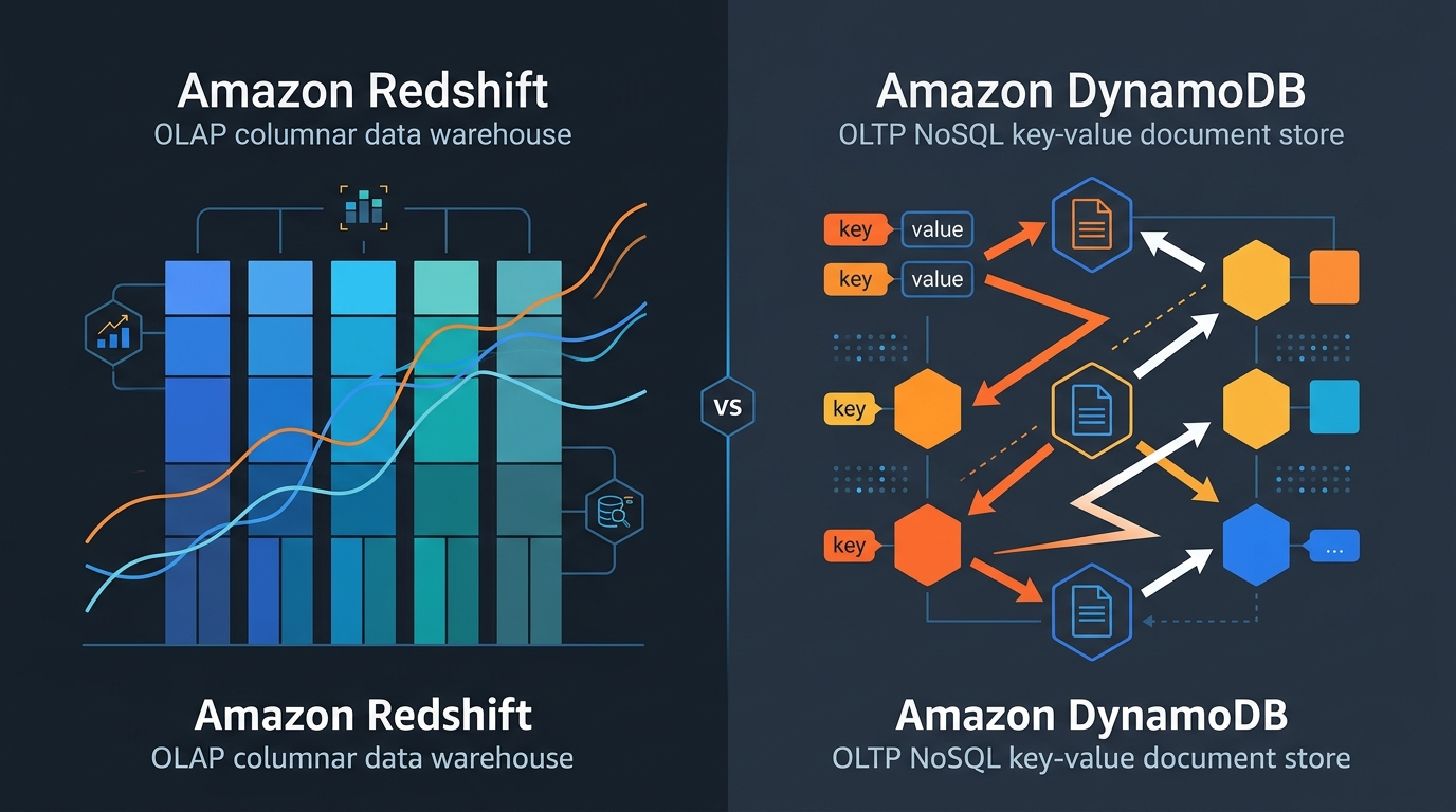
Most “Redshift vs DynamoDB” comparisons are built on a false premise — that these two services are alternatives to each other. They are not. Amazon Redshift is an OLAP data warehouse; DynamoDB is an OLTP key-value and document store. Choosing between them should take about thirty seconds once you understand what each one is designed to do.
The more interesting questions in 2026 are the ones that come after that choice. What actually changed with Redshift Serverless and RA3 nodes? How does DynamoDB’s pricing model hold up at scale? When does zero-ETL between the two services make sense? And what about the gray area — Athena, Aurora, and Babelfish?
The fundamental difference: OLAP vs OLTP
Redshift stores data in columns. When you run SELECT SUM(revenue) FROM orders WHERE region = 'us-east' AND date > '2025-01-01', Redshift reads only the revenue, region, and date columns from disk, compressing and scanning them efficiently across billions of rows. The query might touch 500 million records and return in 3 seconds.
DynamoDB stores data as items (rows) with a partition key and optional sort key. A GetItem call retrieves a single item by its exact key in under 10 milliseconds regardless of whether the table has 10,000 items or 10 billion. But SELECT SUM(revenue) WHERE region = 'us-east' on DynamoDB requires either a full table scan (expensive, slow) or a very specific secondary index design that you planned for upfront.
The failure mode I see most often is picking the wrong tool. Teams that design DynamoDB tables for analytics workloads end up with either incomplete data or scan-based queries that consume enormous read capacity and cost multiples of what Redshift would. Teams that try to use Redshift for operational access patterns — serving individual user records to a live application — hit latency floors that make it unusable for sub-100ms SLA requirements. Query startup overhead alone can be 50-200ms on Redshift. That’s a dealbreaker for user-facing APIs.
Redshift in 2026: Serverless, RA3, and zero-ETL
RA3 nodes split compute and storage. You pay for compute nodes (ra3.xlplus, ra3.4xlarge, ra3.16xlarge) and separately for managed storage (AQUA-backed S3 at $0.024/GB-month). This matters because you can scale compute independently of how much data you have stored. Historically, Redshift’s dense compute nodes required you to add more storage every time you needed more CPU. RA3 eliminates that coupling.
ra3.xlplus at $1.086/hr per node is the starting point for most production workloads. A two-node ra3.xlplus cluster handles datasets in the hundreds of GB range comfortably. For TB-scale analytics with complex multi-table joins, ra3.4xlarge ($3.26/hr) becomes relevant.
Redshift Serverless launched in 2022 and has matured significantly — I was skeptical when it first came out, but it’s genuinely good now. You get a namespace and workgroup, specify a base capacity in Redshift Processing Units (RPUs, 8-512 RPU), and pay $0.36 per RPU-hour. The cluster scales automatically based on query complexity and concurrency.
For teams running analytics intermittently — nightly ETL jobs, weekly BI reports, ad-hoc data science queries — Serverless eliminates idle costs. A cluster that runs 4 hours per day at 32 RPU costs 32 × 4 × 30 × $0.36 = $1,382/month vs. a 2-node ra3.xlplus cluster running 24/7 at $0.372/hr × 720h = $1,564/month. The savings are modest for continuous workloads but meaningful for intermittent ones.
Zero-ETL integrations are the genuinely new thing in Redshift. AWS launched zero-ETL from Aurora MySQL to Redshift in 2023, from Aurora PostgreSQL in 2024, and from DynamoDB to Redshift in late 2023. The integration replicates data continuously — changes appear in Redshift typically within seconds to minutes — without you writing or maintaining any pipeline code.
This changes a common architecture pattern I’ve seen at a lot of teams. Previously, the path from a transactional Aurora database to Redshift analytics ran through DMS, Firehose, or a custom Lambda pipeline. Zero-ETL replaces that with a native AWS feature that requires no infrastructure to maintain. There are limitations (Aurora must run on supported instance classes, the target Redshift cluster must be provisioned rather than Serverless for some integrations), but for the standard Aurora → Redshift analytics pipeline, zero-ETL is now the right default.
DynamoDB in 2026: pricing, global tables, and streams
DynamoDB’s pricing model hasn’t changed structurally, but understanding it correctly matters more as workloads scale.
On-demand mode charges per request: $1.25 per million write request units (WRU) and $0.25 per million read request units (RRU) in us-east-1. One WRU handles writes up to 1KB; one RRU handles eventually consistent reads up to 4KB. A transactional write costs 2 WRUs. A strongly consistent read costs 2 RRUs.
Provisioned mode charges for reserved capacity: $0.00065 per write capacity unit (WCU) per hour and $0.00013 per RCU per hour. At sustained high throughput, provisioned capacity is substantially cheaper than on-demand. A table handling 1,000 writes/second continuously costs:
- On-demand: 1,000 × 3,600 × 24 × 30 × $0.00000125 = $162/month
- Provisioned (1,000 WCU): 1,000 × 720h × $0.00065 = $468/month
On-demand is cheaper here. That reversal happens because provisioned charges per reserved unit per hour regardless of utilization, while on-demand charges per actual request. For tables with variable traffic, on-demand almost always wins unless you can predict and sustain very high steady-state utilization. Auto Scaling helps with provisioned mode but adds complexity.
Global Tables in 2026 replicate to up to 8 regions with typically under 1-second replication lag. Write costs are multiplied by the number of regions — a table replicated to 3 regions effectively triples your write cost. Read costs are per-region and not multiplied. For global applications where users need local-region writes with millisecond latency, Global Tables removes what used to require complex custom replication logic.
DynamoDB Streams captures item-level changes in order, per partition, with a 24-hour retention window. Common uses: triggering Lambda to sync changes downstream, feeding Kinesis Data Streams for analytics, and the zero-ETL integration with Redshift (which is built on Streams under the hood).
For Cassandra-compatible workloads that need the DynamoDB operational model, Amazon Keyspaces is worth understanding — it uses the same CQL interface while providing comparable managed-service guarantees.
When to use Redshift
My default recommendation for analytics is Redshift when the data volume is in the tens of GB to petabyte range and queries need to aggregate across it. Columnar compression typically achieves 3-5x compression ratios, so 1TB of raw data occupies 200-333GB of actual storage.
It’s also the right call when the team works in SQL. Redshift supports a broad SQL dialect, window functions, lateral joins, and connects directly to BI tools like Tableau, Looker, QuickSight, and PowerBI via JDBC/ODBC. The barrier to productive analytics is low for anyone who knows SQL.
Redshift really shines when query patterns are not known in advance. In DynamoDB, every access pattern must be anticipated and designed into the key schema or secondary indexes. In Redshift, you write whatever SQL makes sense for the question you’re answering today.
Historical data analysis is native territory for Redshift. The columnar format, zone maps, and sort keys are built for range scans on time-series data. Queries like “show me all orders from Q3 2024 where discount exceeded 20%, grouped by product category” are exactly what it’s optimized for.
When to use DynamoDB
DynamoDB is the right answer when latency must be in single-digit milliseconds and the access pattern is by known key. User profiles, session data, order status, device state, IoT sensor readings — any workload where you know the exact key at read time and need a sub-10ms response.
It also works well when the schema is fluid or variable per item. Redshift requires fixed columns. DynamoDB items in the same table can have completely different attributes — some items have 3 attributes, others have 40. This flexibility suits evolving product data models.
For genuinely large and unpredictable scale, DynamoDB is hard to beat operationally. It handles millions of requests per second without you touching a configuration dial. There’s no concept of a connection pool, no query planner to tune, no vacuum process to manage. For serverless architectures (Lambda + API Gateway + DynamoDB), the operational surface is minimal.
DynamoDB Streams + Lambda is also a well-worn pattern for event-driven workloads — inventory updates triggering notifications, order status changes propagating to fulfillment systems, user activity feeding a recommendation pipeline. I’ve seen teams build surprisingly complex event meshes on top of this combination.
The gray area: Athena, Aurora Babelfish, and when neither is right
Amazon Athena queries data in S3 directly using standard SQL. It costs $5 per TB scanned and requires no cluster. For ad-hoc analytics on data already living in S3 (CloudTrail logs, application logs, data lake exports), Athena is often cheaper than Redshift for infrequent queries. The tradeoff: query latency is higher (10-60 seconds for complex queries vs. 1-5 seconds on Redshift), and without careful partitioning and columnar formats (Parquet, ORC), costs escalate quickly.
Aurora with Babelfish provides T-SQL compatibility on a PostgreSQL engine. It doesn’t compete with Redshift for analytics, but it blurs the line for teams migrating from SQL Server who need both transactional and moderate analytical capabilities. Aurora handles OLTP at Redshift’s OLAP capability boundary — complex aggregations on hundreds of millions of rows will hit limits, but aggregations on millions of rows with good index design are fine.
The DynamoDB zero-ETL to Redshift integration is where these two services actually complement each other rather than compete. The operational pattern: DynamoDB serves your live application at millisecond latency, zero-ETL replicates those writes to Redshift with minimal lag, and your data team runs analytics queries on Redshift without touching the production DynamoDB table. This separation of operational and analytical workloads was previously expensive to build and maintain. Zero-ETL makes it a configuration choice.
Cost example: 100GB of analytics data
For a concrete comparison, consider 100GB of analytics data queried an average of 10 times per day by a 5-person data team.
Redshift Serverless (32 RPU base, ~1hr/query session):
10 query sessions/day × 1hr × 32 RPU × $0.36 = $115.20/day → $3,456/month
Storage: 100GB at roughly 25GB after compression × $0.024/GB-month = $0.60/month
Total: ~$3,457/month
Redshift Serverless with smarter RPU (16 RPU for small team):
10 × 1hr × 16 RPU × $0.36 = $57.60/day → $1,728/month + storage = ~$1,729/month
Athena (data in Parquet on S3, well-partitioned):
Assume each query scans 5GB after partition pruning: 10 queries/day × 5GB × $0.000005/GB = $0.25/day → $7.50/month
S3 storage: 100GB raw → ~30GB in Parquet × $0.023/GB-month = $0.69/month
Total: ~$8/month
DynamoDB (wrong tool, but for reference):
Storing 100GB of analytics data: ~$25/month storage. Reading it for analytics requires full table scans — at 1KB average item size, 100GB = 100M items, 50M RRUs per full scan × 10 scans/day = 500M RRUs × $0.000000025 = $12.50/day → $375/month just in read costs, with no aggregation capability.
Athena on well-structured Parquet data wins on cost by a wide margin for infrequent, ad-hoc analytics. Redshift wins when queries are frequent, the team needs faster interactive response times, or the data volume grows beyond what Athena handles efficiently. DynamoDB should not be used here at all.
For the cost optimization frameworks that govern these decisions, see AWS FinOps in 2026.
Decision table
| Axis | Choose Redshift | Choose DynamoDB |
|---|---|---|
| Query pattern | Aggregations, range scans, multi-table JOINs, ad-hoc SQL | Point reads/writes by known key, predictable access patterns |
| Latency requirement | Seconds acceptable (analytics, BI dashboards) | Single-digit milliseconds required (user-facing, APIs) |
| Team SQL fluency | High — analysts and data engineers on staff | Low SQL fluency OK — SDK-based access, no joins needed |
| Data volume | GB to petabyte range, analytical datasets | Any volume — scales from KB to PB of items |
| Schema flexibility | Fixed schema, evolves with ALTER TABLE | Schema-less per item, attributes vary freely |
| Operational overhead | Low with Serverless, moderate with provisioned RA3 | Near-zero — fully managed, no capacity tuning with on-demand |
| Cost model | RPU-hours (Serverless) or node-hours (provisioned) | Per request (on-demand) or reserved capacity (provisioned) |
| Integration path | Aurora zero-ETL, S3, Kinesis, direct JDBC/ODBC | Streams → Lambda, zero-ETL → Redshift, Kinesis, EventBridge |
These two services are most powerful together. Use DynamoDB as the operational store — serving live application traffic at predictable millisecond latency — and Redshift as the analytical layer, fed via zero-ETL or Streams-based pipelines, where the data team can query freely without impacting production. That combination covers a very large fraction of what modern data-driven applications need, and the zero-ETL integration makes it much less painful to wire up than it used to be.
For caching in front of either service, Amazon ElastiCache with Valkey handles session data and hot-key acceleration with sub-millisecond response times, completing the typical AWS data tier stack.
Explore more like this

Aurora Serverless v2 + Bedrock: AI Database Queries in 2026
I connected Bedrock to our Aurora cluster last month. The first thing I asked it was “show me all customers who churned in Q1 but came back in Q2” —...
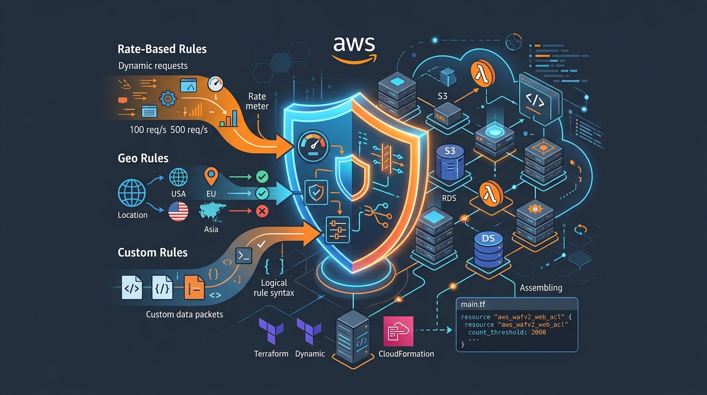
AWS WAF Rules Deep Dive: Rate-Based, Geo, and Custom Rules
WAF is one of those services where the default managed rules get you 80% of the way there. The last 20% is where it gets interesting.

Comments